The Context
This is the second post of a series (previously part 1, next comes part 3 and part 4) discussing our epistemological access to Pr(H|E) and whether Bayes theorem is always the most reliable way to find it. In the last post I provided a mathematical example in which Pr(H|E) cannot be found via Bayes but can be found another way. Here I discuss whether the same situation holds for cases where H is a hypothesis and E is some sort of evidence.
Bayesian Diaganosis
If we consider the textbook example of Bayes at work—medical diagnosis—we find a situation where we need Bayes to find Pr(H|E). In this case H (i.e. H+) = a person having the dreaded disease H (take your pick, Hansen’s, Hashimoto’s, Hepatitis, etc.) and E+ stands for having a positive test result. What information do we have? 1) the background frequency of a disease, 2) how often the test correctly detects the disease, and 3) how often the test is positive when there is no disease. Here’s a set of diagrams that helps illustrate how this works.
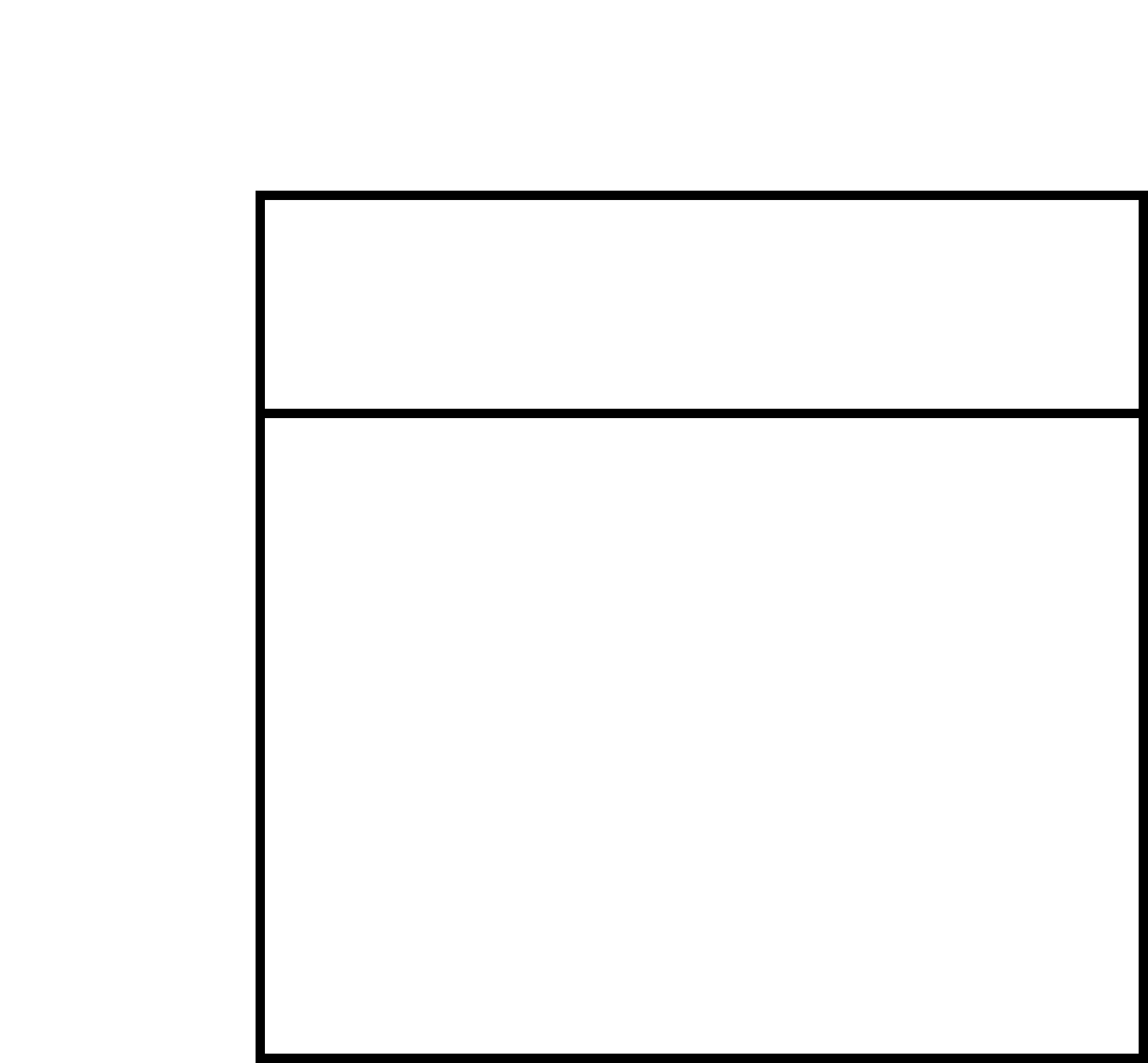
The first chart shows the result of a study trying to find the percentage of people in a population that has the dreaded disease H. The investigators randomly selected a certain number of people from the population and find how many of their subjects have H or don’t have H. Given census data about the total number of people in in the population, and an assumption that the tested population accurately represents the total population, we can find Pr(H)– i.e., the probability that a random member of the population has disease H. In our diagram we see that approximately ¼ of the population has H and ¾ does not. So here Pr(H+) = .25
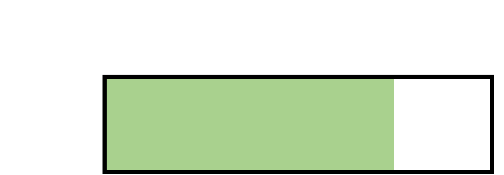
However, this study doesn’t tell us anything about E, the results of a certain test for H. For this we turn to a separate study. In this case we are looking at a rapid test and seeing how accurate it is. To do this we take a population that we already know has dreaded disease H and see how often it gives positive test results. This diagram shows the results. So out of a group where everyone has the disease (H+), the test accurately has a positive result (E+) about ¾ of the time, giving us Pr(E+|H+) = .75.
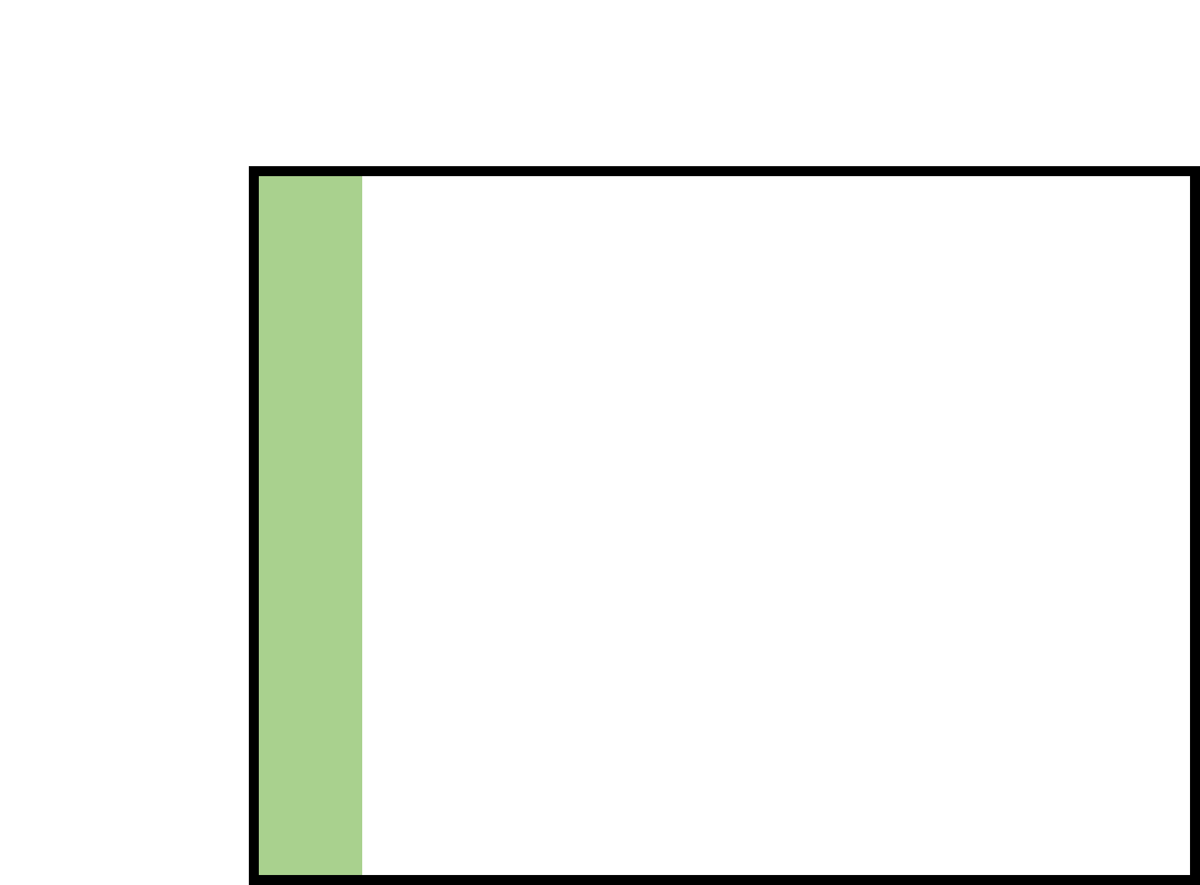
However, knowing how often the test registers positive whent the disease is present is not enough. We need to find not only how the test does with people who have the disease, but also how it does with those who don’t have the disease. (the false positive rate) In this case we see that out of a population that doesn’t have the disease the test comes back positive 1/10 times. This gives us Pr(E+|H-) = .1.
This now gives us everything we need to fill out the graph and find Pr(H|E). When we put the pieces of the graph together we can see that we have to ability to see how H+, H-, E+, and E- all relate to each other. Critically, it now also lets us find Pr(E), which is the denominator in Bayes theorem. In this graph, Pr(E) is the percentage of the graph that is green. Mathematically, it is the (green area) / (total area). But how do we find this?
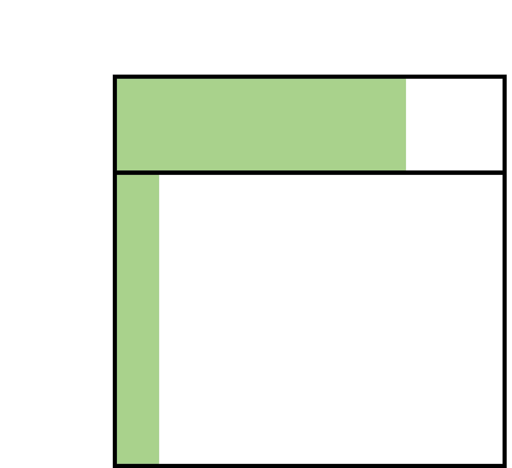
Well, we know how much of the H+ box is green and we also know how much of the total area the H+ box takes up. Basically, if we know how much of a slice of pie I ate, and I know how many slices there are in the whole pie, I can figure out how much of the whole pie I ate. In our case, since ¾ of the H+ pie is green, and H+ is ¼ of the total pie, we can multiply these together to find what percentage of the total pie in the H+ slice is green: ¾ x ¼ = 3/16 = .1875. However, to find how much of the total pie is green (E+) we have to count the green in the H- section as well. Since 1/10 of H- is green and H- is ¾ of the total pie then the green in H- makes up 3/40 = .075 of the total pie. All we need to do to find the total percentage of green, Pr(E), is add these together .1875 + .075 = .2625. If we write this mathematically we get Pr(E+) = Pr(E+|H+) Pr(H+) + Pr(E|H-) Pr(H-).
When we put all of our numbers together in Bayes Theorem we get:

This means that when Jack tests positive, it raised his chances of having H from 25% (the base percentage any member of the population has H) to 71.43%.
Note that here we have put together analyses of three different groups. First is the group that was studied to find the ratio of H to the total; the result of this is generalized to give us the percentage of the whole population that suffers from the disease, Pr(H+). The second was the group of ill people that we gave the test to that allowed us to find Pr(E+|H+). And third, there was the group of well people that allowed us to find Pr(E+|H-).
Non-Bayesian Diaganosis
While this is the classic diagnosis example, does the search for Pr(H|E) require this pattern? Not necessarily. Consider a different example that uses the same numbers, but has a different epistemological position. H still indicates having (or not) disease, and E indicates the result of a test. But in this case, we are dendrologists looking after a very endangered species. The extant trees of this species are under our care in our conservation park. A real problem with this species is its susceptibility to blight. If caught early enough the host can be saved, but too late and the tree dies with a distinctive orange-brown bloom of doom.
A new test was developed to help catch the blight earlier while it’s still treatable. A study was done where each tree was tested, the results logged, and then each tree watched to see if the blight developed. As it turns out, 26.25% of the trees tested positive, i.e. Pr(E+) = .2625.
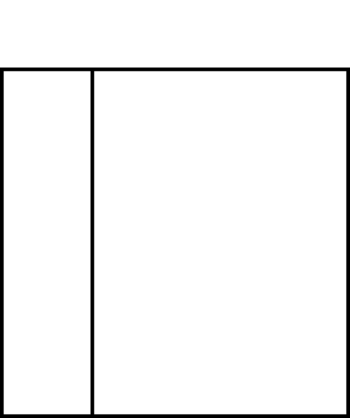
The scientists also noted that 18.75% (3/16’ths) of the total number of trees tested positive and then developed the baleful blight Pr(H∩E) = 18.75%. This now allows us to shade in the area that is both H+ and also E+. This is made possible by means of the definition of conditional probability, i.e., the probability of the conjunction of A and B, Pr(A∩B), divided by the probability of B, Pr(B), Pr(A∩B)/Pr(B) = Pr(A|B). In our case this means that Pr(H+|E+) = Pr(H+∩E+) / Pr(E+). We have both these values already in hand and so Pr(H+|E+) = .1875 / .2625 = .7143. Note that this is same value as in the previous example, exactly as it should be.
Note also we did this without having to find the priors, Pr(H+) and Pr(H-), or the likelihoods Pr(E+|H+), Pr(E+|H-). In this case they can’t even be calculated because we don’t know how much of H+ and H- are in the E- space. So in this case, when we receive a positive result on the blight test for our tree, we can move right past Bayes and just use the conditional probability formula and discover that there is a 71.43% chance of that tree having blight. In this case all that is needed is Pr(E+) and Pr(H+∩E+).
However, in a similar scenario, one does not even need this much information. The previous only works if the total size of the population is known. Pr(H+∩E+) is the percentage of things that are both H and E compared to the total population. Similarly, Pr(E+) is a ratio of things compared to the total population. But what happens when the size of Pr(E-) is unknown, like in the first bunny example? Here this could happen if the foresters only kept track of the positive test results but not the negatives. Has this negligence ruined our chances to find Pr(H|E)? If the actual numbers are retained, the answer is no, Pr(H|E) is still attainable.
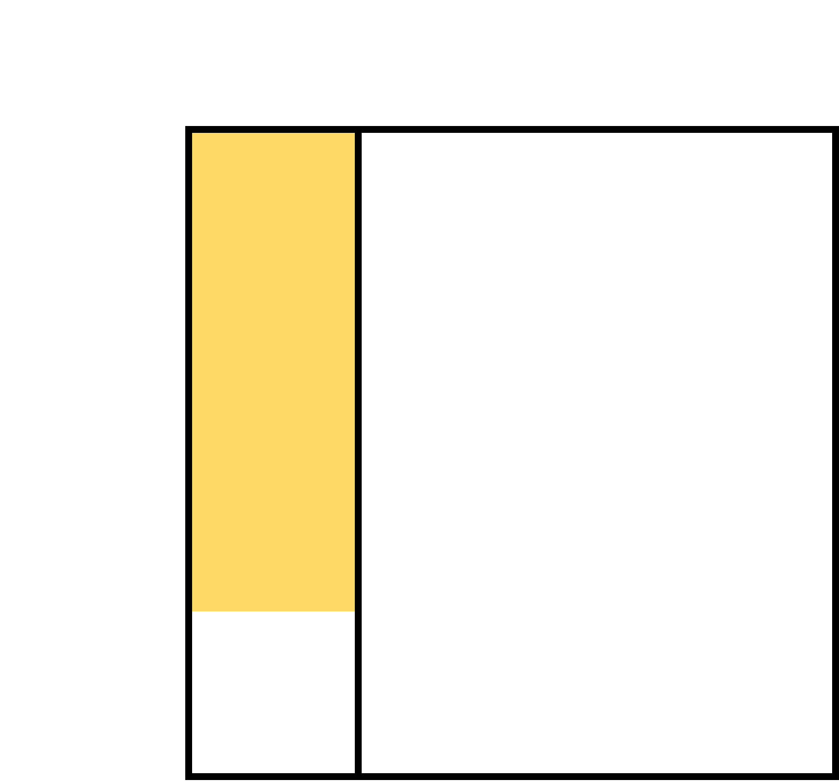
Let’s assume our dendrologists are now looking at bushes, and they only kept track of positive tests and which of those positive test plants got sick. Suppose that out of an unknown number of tests 100 came back positive and of those positive tests 71 of the bushes got sick (this just rounds the numbers above). This would give us a diagram like this.
In this case we don’t know E-, H-, H+, or the total. However, the ‘posterior’ probability is still known here, Pr(H+|E+) = .71. Now you might wonder how this is possible since conditional probability is defined as Pr(H|E) = Pr(H∩E) / Pr(E) — a situation which seems to require the total population, as noted above. However, recall that the probability of E, Pr(E+), is simply the number of E+ things divided by the total number of things. But the total number is simply the sum of E things and non-E things. Similarly, Pr(H∩E) is simply the number of things that are both H+ and E+ divided by the total (i.e. the sum of E+ and E- things). When all of this gets put into an equation it becomes clear why the total number of things is not needed here.
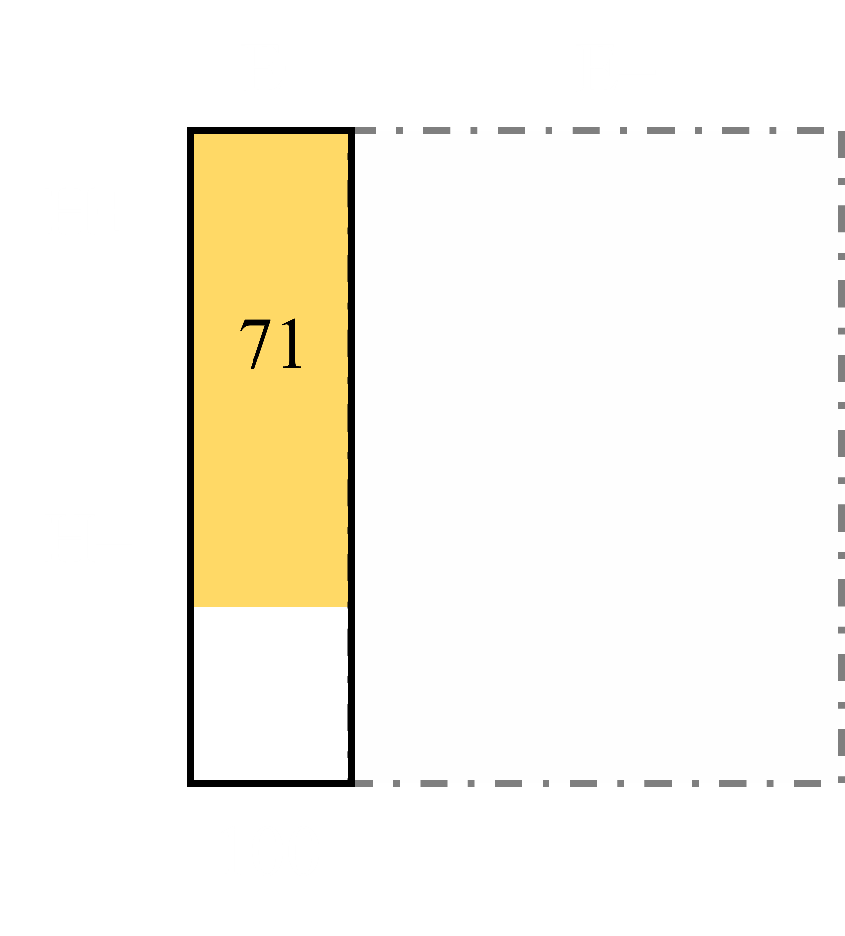
We see that after the equation is reduced, the totals cancel out and Pr(H|E) reduces to the number of things that are both H and E to the number of things that are E. Hence, in the bush example Pr(H|E) = 71/100 = .71.
So what can we conclude from this? First, we can still find Pr(H|E) in cases where we are dealing with hypotheses and evidence without Bayes theorem. Second, moving to Pr(H|E) more directly as a conditional probability requires epistemological access to both H∩E and E (or their probabilities). Without these one must take another route—such as the Bayesian one. This explains why it didn’t work with our medical example. The first study didn’t provide Pr(H∩E), the number/ratio of people who were ill and also tested positive. The second study gave us that but it didn’t tell us Pr(E). We don’t know how many people tested positive compared to the total number of people. In order to find that it required the third study. To skip Bayes one needs to have a well-defined E, and access to H∩E. In cases where this is true, one doesn’t need Bayes.
Now that we’ve worked through conditional probabilities, it’s time to apply them to Biblical Studies in the next post.